- Momentum transport deals with the transport of momentum in fluids and is also known as fluid dynamics.
- Energy transport deals with the transport of different forms of energy in a system and is also known as heat transfer.
- Mass transport deals with the transport of various chemical species themselves.
Three different types of physical quantities are used in transport phenomena: scalars (e.g. temperature, pressure and concentration), vectors (e.g. velocity, momentum and force) and second order tensors (e.g. stress or momentum flux and velocity gradient). It is essential to have a primary knowledge of the mathematical operations of scalar, vector and tensor quantities for solving the problems of transport phenomena. In fact, the use of the indicial notation in cartesian coordinates will enable us to express the long formulae encountered in transport phenomena in a concise and compact fashion. In addition, any equation written in vector tensor form is equally valid in any coordinate system.
In this course, we will using the following notations for scalar, vector and tensor quantities:
Notations:
|
a,b,c |
scalar quantities |
 |
vector quantities |
|
 |
2nd order tensor quantities |
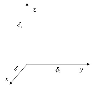
Here,  and
and ![]() are the unit vectors in x, y and z direction respectively.
are the unit vectors in x, y and z direction respectively.
Most of us might have already encountered scalars and vectors in the study of high-school physics. It was pointed out that the vectors also have a direction associated with them along with a magnitude, whereas scalars only have a magnitude but no direction. Extending this definition, we can loosely define a 2nd order tensor as a physical quantity which has a magnitude and two different directions associated with it. To better understand, why we might need two different directions for specifying a particular physical quantity. Let us take the example of the stresses which may arise in a solid body, or in a fluid. Clearly, the stresses are associated with magnitude of forces, as well as with an area, whose direction is also need to be specified by the outward normal to the face of the area on which a particular force acting. Hence, we will require 32, i.e., 9 components to specify a stress completely in a 3 dimensional cartesian coordinate system. In general, an nth order tensor will be specified by 3n components (in a 3-dimensional system). However, the number of components alone cannot determine whether a physical quantity is a vector or a tensor. The additional requirement is that there should be some transformation rule for obtaining the corresponding tensors when we rotate the coordinate system about the origin. Thus, the tensor quantities can be defined by two essential conditions:
- These quantities should have 3n components. According to this definition, scalar quantities are zero order tensors and have 30= 1 component. Vector quantities are first order tensors and have 31 = 3 components. Second order tensors have 32 = 9 components and third order tensors have 33 = 27 components. Third and higher order tensors are not used in transport phenomena, and are not dealt here.
- The second necessary requirement of any tensor quantity is that it should follow some transformation rule.
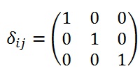
It is expressed as a symbol δij
δij=0, if i≠j
- εijk=0 if any two of indices i, j, k are equal. For example ε113,ε131,ε111,ε222=0
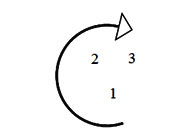
- εijk=+1 when the indices i, j, k are different and are in cyclic order (123), For example ε123
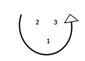
- εijk=-1 when the indices i, j, k are different and are in anti-cyclic order. For example ε321
Free indices are the indices which occur only once in each tensor term. For example, i is the free index in following expression vij wj
Any free indices in a tensorial expression can be replaced by any other indices as long as this symbol has not already occurred in the expression. For example, Aij Bj= CiDjEj is equivalent to Akj Bj= CkDjEj.
Any dummy index implies the summation of all components of that tensor term associated with each coordinate axis. Thus, when we write Aiδi, we actually imply  .
.
Any dummy index in a tensor term can be replaced by any other symbol as long as this symbol has not already occurred in previous terms. For example, Aijkδjδk= Aipqδpδq.
Note: The dummy indices can be renamed in each term separately in a equations but free indices should be renamed for all terms in a tensor equations. For example, Aij Bj= CiDjEj can be replaced by Akp Bp= CkDjEj.
 can be simply written as εijkεljk . Since j and k are repeating, there is no need to write summation sign over these indices